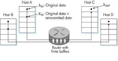
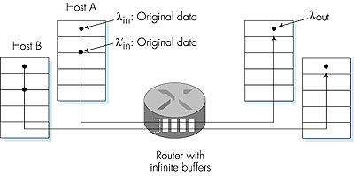
In this section, we consider the problem of congestion control in a general context, seeking to understand why congestion is a "bad thing," how network congestion is manifested in the performance received by upper-layer applications, and various approaches that can be taken to avoid, or react to, network congestion. This more general study of congestion control is appropriate since, as with reliable data transfer, it is high on the "top-10" list of fundamentally important problems in networking. We conclude this section with a discussion of congestion control in the ABR service in asynchronous transfer mode (ATM) networks. The following section contains a detailed study of TCP's congestion-control algorithm. 

3.6.1: The Causes and the Costs of Congestion

Scenario 1: Two Senders, a Router with Infinite Buffers

We begin by considering perhaps the simplest congestion scenario possible: two hosts (A and B) each have a connection that shares a single hop between source and destination, as shown in Figure 3.41. 

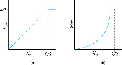
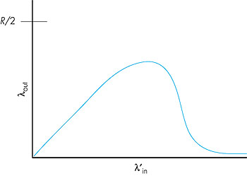
Let's assume that the application in Host A is sending data into the connection (for example, passing data to the transport-level protocol via a socket) at an average rate of _in bytes/sec. These data are "original" in the sense that each unit of data is sent into the socket only once. The underlying transport-level protocol is a simple one. Data is encapsulated and sent; no error recovery (for example, retransmission), flow control, or congestion control is performed. Host B operates in a similar manner, and we assume for simplicity that it too is sending at a rate of _in bytes/sec. Packets from hosts A and B pass through a router and over a shared outgoing link of capacity R. The router has buffers that allow it to store incoming packets when the packet-arrival rate exceeds the outgoing link's capacity. In this first scenario, we'll assume that the router has an infinite amount of buffer space. 

Figure 3.42 plots the performance of Host A's connection under this first scenario. The left graph plots the per-connection throughput (number of bytes per second at the receiver) as a function of the connection sending rate. For a sending rate between 0 and R/2, the throughput at the receiver equals the sender's sending rate--everything sent by the sender is received at the receiver with a finite delay. When the sending rate is above R/2, however, the throughput is only R/2. This upper limit on throughput is a consequence of the sharing of link capacity between two connections. The link simply cannot deliver packets to a receiver at a steady-state rate that exceeds R/2. No matter how high Hosts A and B set their sending rates, they will each never see a throughput higher than R/2. 

Achieving a per-connection throughput of R/2 might actually appear to be a "good thing," as the link is fully utilized in delivering packets to their destinations. The right-hand graph in Figure 3.42, however, shows the consequences of operating near link capacity. As the sending rate approaches R/2 (from the left), the average delay becomes larger and larger. When the sending rate exceeds R/2, the average number of queued packets in the router is unbounded, and the average delay between source and destination becomes infinite (assuming that the connections operate at these sending rates for an infinite period of time). Thus, while operating at an aggregate throughput of near R may be ideal from a throughput standpoint, it is far from ideal from a delay standpoint. Even in this (extremely) idealized scenario, we've already found one cost of a congested network--large queuing delays are experienced as the packet-arrival rate nears the link capacity.

Scenario 2: Two Senders, a Router with Finite Buffers

Let us now slightly modify scenario 1 in the following two ways (see Figure 3.43). First, the amount of router buffering is assumed to be finite. Second, we assume that each connection is reliable. If a packet containing a transport-level segment is dropped at the router, it will eventually be retransmitted by the sender. Because packets can be retransmitted, we must now be more careful with our use of the term "sending rate." Specifically, let us again denote the rate at which the application sends original data into the socket by _in bytes/sec. The rate at which the transport layer sends segments (containing original data or retransmitted data) into the network will be denoted _in' bytes/sec. _in' is sometimes referred to as the offered load to the network. 

The performance realized under scenario 2 will now depend strongly on how retransmission is performed. First, consider the unrealistic case that Host A is able to somehow (magically!) determine whether or not a buffer is free in the router and thus sends a packet only when a buffer is free. In this case, no loss would occur, _in would be equal to _in', and the throughput of the connection would be equal to _in. This case is shown by the upper curve in Figure 3.44(a). From a throughput standpoint, performance is ideal--everything that is sent is received. Note that the average host sending rate cannot exceed R/2 under this scenario, since packet loss is assumed never to occur. 

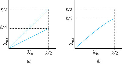
Consider next the slightly more realistic case that the sender retransmits only when a packet is known for certain to be lost. (Again, this assumption is a bit of a stretch. However, it is possible that the sending host might set its timeout large enough to be virtually assured that a packet that has not been acknowledged has been lost.) In this case, the performance might look something like that shown in Figure 3.44(b). 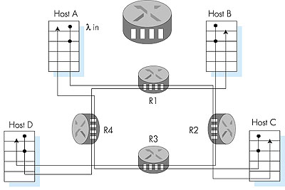To appreciate what is happening here, consider the case that the offered load, _in' (the rate of original data transmission plus retransmissions), equals 0.5R. According to Figure 3.44(b), at this value of the offered load, the rate at which data are delivered to the receiver application is R/3. Thus, out of the 0.5R units of data transmitted, 0.333R bytes/sec (on average) are original data and 0.266R bytes per second (on average) are retransmitted data. We see here another cost of a congested network--the sender must perform retransmissions in order to compensate for dropped (lost) packets due to buffer overflow.

Finally, let us consider the case that the sender may timeout prematurely and retransmit a packet that has been delayed in the queue, but not yet lost. In this case, both the original data packet and the retransmission may both reach the receiver. Of course, the receiver needs but one copy of this packet and will discard the retransmission. In this case, the "work" done by the router in forwarding the retransmitted copy of the original packet was "wasted," as the receiver will have already received the original copy of this packet. The router would have better used the link transmission capacity to send a different packet instead. Here then is yet another cost of a congested network--unneeded retransmissions by the sender in the face of large delays may cause a router to use its link bandwidth to forward unneeded copies of a packet. The lower curve in Figure 3.44(a) shows the throughput versus offered load when each packet is assumed to be forwarded (on average) twice by the router. Since each packet is forwarded twice, the throughput achieved will be given by the line segment in Figure 3.44(a) with the asymptotic value of R/4. 

Scenario 3: Four Senders, Routers with Finite Buffers, and Multihop Paths

In our final congestion scenario, four hosts transmit packets, each over overlapping two-hop paths, as shown in Figure 3.45. We again assume that each host uses a timeout/ retransmission mechanism to implement a reliable data transfer service, that all hosts have the same value of _in, and that all router links have capacity R bytes/sec. 

Let us consider the connection from Host A to Host C, passing through Routers R1 and R2. The A-C connection shares router R1 with the D-B connection and shares router R2 with the B-D connection. For extremely small values of _in, buffer overflows are rare (as in congestion scenarios 1 and 2), and the throughput approximately equals the offered load. For slightly larger values of _in, the corresponding throughput is also larger, as more original data is being transmitted into the network and delivered to the destination, and overflows are still rare. Thus, for small values of _in, an increase in _in results in an increase in _out. 

Having considered the case of extremely low traffic, let us next examine the case that _in (and hence _in') is extremely large. Consider router R2. The A-C traffic arriving to router R2 (which arrives at R2 after being forwarded from R1) can have an arrival rate at R2 that is at most R, the capacity of the link from R1 to R2, regardless of the value of _in. If _in' is extremely large for all connections (including the B-D connection), then the arrival rate of B-D traffic at R2 can be much larger than that of the A-C traffic. Because the A-C and B-D traffic must compete at router R2 for the limited amount of buffer space, the amount of A-C traffic that successfully gets through R2 (that is, is not lost due to buffer overflow) becomes smaller and smaller as the offered load from B-D gets larger and larger. In the limit, as the offered load approaches infinity, an empty buffer at R2 is immediately filled by a B-D packet, and the throughput of the A-C connection at R2 goes to zero. This, in turn, implies that the A-C end-end throughput goes to zero in the limit of heavy traffic. These considerations give rise to the offered load versus throughput tradeoff shown in Figure 3.46. 

The reason for the eventual decrease in throughput with increasing offered load is evident when one considers the amount of wasted "work" done by the network. In the high-traffic scenario outlined above, whenever a packet is dropped at a second-hop router, the "work" done by the first-hop router in forwarding a packet to the second-hop router ends up being "wasted." The network would have been equally well off (more accurately, equally bad off) if the first router had simply discarded that packet and remained idle. More to the point, the transmission capacity used at the first router to forward the packet to the second router could have been much more profitably used to transmit a different packet. (For example, when selecting a packet for transmission, it might be better for a router to give priority to packets that have already traversed some number of upstream routers.) So here we see yet another cost of dropping a packet due to congestion--when a packet is dropped along a path, the transmission capacity that was used at each of the upstream routers to forward that packet to the point at which it is dropped ends up having been wasted.

3.6.2: Approaches toward Congestion Control

At the broadest level, we can distinguish among congestion-control approaches based on whether or not the network layer provides any explicit assistance to the transport layer for congestion-control purposes: 

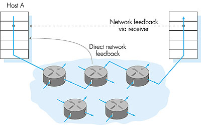
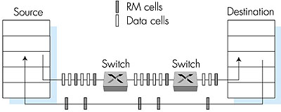
• End-end congestion control. In an end-end approach toward congestion control, the network layer provides no explicit support to the transport layer for congestion-control purposes. Even the presence of congestion in the network must be inferred by the end systems based only on observed network behavior (for example, packet loss and delay). We will see in Section 3.7 that TCP must necessarily take this end-end approach toward congestion control, since the IP layer provides no feedback to the end systems regarding network congestion. TCP segment loss (as indicated by a timeout or a triple duplicate acknowledgment) is taken as an indication of network congestion and TCP decreases its window size accordingly. We will also see that new proposals for TCP use increasing round-trip delay values as indicators of increased network congestion. 
• Network-assisted congestion control. With network-assisted congestion control, network-layer components (that is, routers) provide explicit feedback to the sender regarding the congestion state in the network. This feedback may be as simple as a single bit indicating congestion at a link. This approach was taken in the early IBM SNA [Schwartz 1982] and DEC DECnet [Jain 1989; Ramakrishnan 1990] architectures, was recently proposed for TCP/IP networks [Floyd TCP 1994; RFC 2481], and is used in ATM available bit-rate (ABR) congestion control as well, as discussed below. More sophisticated network-feedback is also possible. For example, one form of ATM ABR congestion control that we will study shortly allows a router to explicitly inform the sender of the transmission rate it (the router) can support on an outgoing link.

3.6.3: ATM ABR Congestion Control

Figure 3.48 shows the framework for ATM ABR congestion control. In our discussion below we adopt ATM terminology (for example, using the term "switch" rather than "router," and the term "cell" rather than "packet"). With ATM ABR service, data cells are transmitted from a source to a destination through a series of intermediate switches. Interspersed with the data cells are so-called resource-management cells, RM cells; we will see shortly that these RM cells can be used to convey congestion-related information among the hosts and switches. When an RM cell is at a destination, it will be "turned around" and sent back to the sender (possibly after the destination has modified the contents of the RM cell). It is also possible for a switch to generate an RM cell itself and send this RM cell directly to a source. RM cells can thus be used to provide both direct network feedback and network-feedback-via-the-receiver, as shown in Figure 3.48. 

ATM ABR congestion control is a rate-based approach. That is, the sender explicitly computes a maximum rate at which it can send and regulates itself accordingly. ABR provides three mechanisms for signaling congestion-related information from the switches to the receiver: 

• EFCI bit. Each data cell contains an EFCI (explicit forward congestion-indication) bit. A congested network switch can set the EFCI bit in a data cell to 1 to signal congestion to the destination host. The destination must check the EFCI bit in all received data cells. When an RM cell arrives at the destination, if the most recently received data cell had the EFCI bit set to 1, then the destination sets the congestion-indication bit (the CI bit) of the RM cell to 1 and sends the RM cell back to the sender. Using the EFCI in data cells and the CI bit in RM cells, a sender can thus be notified about congestion at a network switch. 
• CI and NI bits. As noted above, sender-to-receiver RM cells are interspersed with data cells. The rate of RM cell interspersion is a tunable parameter, with one RM cell every 32 data cells being the default value. These RM cells have a CI (congestion indication) bit and an NI (no increase) bit that can be set by a congested-network switch. Specifically, a switch can set the NI bit in a passing RM cell to 1 under mild congestion and can set the CI bit to 1 under severe congestion conditions. When a destination host receives an RM cell, it will send the RM cell back to the sender with its CI and NI bits intact (except that CI may be set to 1 by the destination as a result of the EFCI mechanism described above). 
• ER setting. Each RM cell also contains a two-byte ER (explicit rate) field. A congested switch may lower the value contained in the ER field in a passing RM cell. In this manner, the ER field will be set to the minimum supportable rate of all switches on the source-to-destination path.