A TCP connection controls its transmission rate by limiting its number of transmitted-but-yet-to-be-acknowledged segments. Let us denote this number of permissible unacknowledged segments as w, often referred to as the TCP window size. Ideally, TCP connections should be allowed to transmit as fast as possible (that is, to have as large a number of outstanding unacknowledged segments as possible) as long as segments are not lost (dropped at routers) due to congestion. In very broad terms, a TCP connection starts with a small value of w and then "probes" for the existence of additional unused link bandwidth at the links on its end-to-end path by increasing w. A TCP connection continues to increase w until a segment loss occurs (as detected by a timeout or duplicate acknowledgments). When such a loss occurs, the TCP connection reduces w to a "safe level" and then begins probing again for unused bandwidth by slowly increasing w. 

An important measure of the performance of a TCP connection is its throughput--the rate at which it transmits data from the sender to the receiver. Clearly, throughput will depend on the value of w. If a TCP sender transmits all w segments back to back, it must then wait for one round-trip time (RTT) until it receives acknowledgments for these segments, at which point it can send w additional segments. If a connection transmits w segments of size MSS bytes every RTT seconds, then the connection's throughput, or transmission rate, is (w · MSS)/RTT bytes per second. 

Suppose now that K TCP connections are traversing a link of capacity R. Suppose also that there are no UDP packets flowing over this link, that each TCP connection is transferring a very large amount of data and that none of these TCP connections traverse any other congested link. Ideally, the window sizes in the TCP connections traversing this link should be such that each connection achieves a throughput of R/K. More generally, if a connection passes through N links, with link n having transmission rate R_n and supporting a total of K_n TCP connections, then ideally this connection should achieve a rate of R_n/K_n on the nth link. However, this connection's end-to-end average rate cannot exceed the minimum rate achieved at all of the links along the end-to-end path. That is, the end-to-end transmission rate for this connection is r = min{R₁/K₁, . . ., R_N/K_N}. We could think of the goal of TCP as providing this connection with this end-to-end rate, r. (In actuality, the formula for r is more complicated, as we should take into account the fact that one or more of the intervening connections may be bottlenecked at some other link that is not on this end-to-end path and hence cannot use their bandwidth share, R_n/K_n. In this case, the value of r would be higher than min{R₁/K₁, . . . , R_N/K_N}. See [Bertsekas 1991].) 

3.7.1: Overview of TCP Congestion Control

The threshold, which we discuss in detail below, is a variable that affects how CongWin grows. 

Let us now look at how the congestion window evolves throughout the lifetime of a TCP connection. In order to focus on congestion control (as opposed to flow control), let us assume that the TCP receive buffer is so large that the receive window constraint can be ignored. In this case, the amount of unacknowledged data that a host can have within a TCP connection is solely limited by CongWin. Further let's assume that a sender has a very large amount of data to send to a receiver. 

Once a TCP connection is established between the two end systems, the application process at the sender writes bytes to the sender's TCP send buffer. TCP grabs chunks of size MSS, encapsulates each chunk within a TCP segment, and passes the segments to the network layer for transmission across the network. The TCP congestion window regulates the times at which the segments are sent into the network (that is, passed to the network layer). Initially, the congestion window is equal to one MSS. TCP sends the first segment into the network and waits for an acknowledgment. If this segment is acknowledged before its timer times out, the sender increases the congestion window by one MSS and sends out two maximum-size segments. If these segments are acknowledged before their timeouts, the sender increases the congestion window by one MSS for each of the acknowledged segments, giving a congestion window of four MSS, and sends out four maximum-sized segments. This procedure continues as long as (1) the congestion window is below the threshold and (2) the acknowledgments arrive before their corresponding timeouts. 

During this phase of the congestion-control procedure, the congestion window increases exponentially fast. The congestion window is initialized to one MSS; after one RTT, the window is increased to two segments; after two round-trip times, the window is increased to four segments; after three round-trip times, the window is increased to eight segments, and so forth. This phase of the algorithm is called slow start because it begins with a small congestion window equal to one MSS. (The transmission rate of the connection starts slowly but accelerates rapidly.) 

The slow-start phase ends when the window size exceeds the value of threshold. Once the congestion window is larger than the current value of threshold, the congestion window grows linearly rather than exponentially. Specifically, if w is the current value of the congestion window, and w is larger than threshold, then after w acknowledgments have arrived, TCP replaces w with w + 1. This has the effect of increasing the congestion window by 1 in each RTT for which an entire window's worth of acknowledgments arrives. This phase of the algorithm is called congestion avoidance.

The congestion-avoidance phase continues as long as the acknowledgments arrive before their corresponding timeouts. But the window size, and hence the rate at which the TCP sender can send, cannot increase forever. Eventually, the TCP rate will be such that one of the links along the path becomes saturated, at which point loss (and a resulting timeout at the sender) will occur. When a timeout occurs, the value of threshold is set to half the value of the current congestion window, and the congestion window is reset to one MSS. The sender then again grows the congestion window exponentially fast using the slow-start procedure until the congestion window hits the threshold. 

In summary: 

• When the congestion window is below the threshold, the congestion window grows exponentially. 
• When the congestion window is above the threshold, the congestion window grows linearly. 
• Whenever there is a timeout, the threshold is set to one-half of the current congestion window and the congestion window is then set to 1.

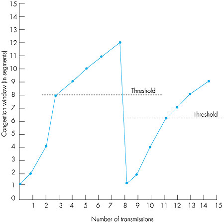
The evolution of TCP's congestion window is illustrated in Figure 3.49. In this figure, the threshold is initially equal to 8 • MSS. The congestion window climbs exponentially fast during slow start and hits the threshold at the third transmission. The congestion window then climbs linearly until loss occurs, just after transmission 7. Note that the congestion window is 12 • MSS when loss occurs. The threshold is then set to 0.5 • CongWin = 6 • MSS and the congestion window is set 1. And the process continues. This congestion-control algorithm is due to V. Jacobson [Jacobson 1988]; a number of modifications to Jacobson's initial algorithm are described in Stevens (1994) and in RFC 2581. 

We note briefly here that the description of TCP slow start is an idealized one. An initial window of up to two MSS's is a proposed standard [RFC 2581] and it is actually used in some implementations. 

A Trip to Nevada: Tahoe, Reno, and Vegas

The TCP congestion-control algorithm just described is often referred to as Tahoe. One problem with the Tahoe algorithm is that, when a segment is lost, the sender side of the application may have to wait a long period of time for the timeout. For this reason, a variant of Tahoe, called Reno, is implemented by most operating systems. Like Tahoe, Reno sets its congestion window to one segment upon the expiration of a timer. However, Reno also includes the fast retransmit mechanism that we examined in Section 3.5. Recall that fast retransmission triggers the transmission of a dropped segment if three duplicate ACKs for a segment are received before the occurrence of the segment's timeout. Reno also employs a fast-recovery mechanism that essentially cancels the slow-start phase after a fast retransmission. The interested reader is encouraged to see [Stevens 1994] and in [RFC 2581] for details. [Cela 2000] provides interactive animations of congestion avoidance, slow start, fast retransmit, and fast recovery in TCP. 

Most TCP implementations currently use the Reno algorithm. There is, however, another algorithm in the literature, the Vegas algorithm, that can improve Reno's performance. Whereas Tahoe and Reno react to congestion (that is, to overflowing router buffers), Vegas attempts to avoid congestion while maintaining good throughput. The basic idea of Vegas is to (1) detect congestion in the routers between source and destination before packet loss occurs and (2) lower the rate linearly when this imminent packet loss is detected. Imminent packet loss is predicted by observing the round-trip times. The longer the round-trip times of the packets, the greater the congestion in the routers. The Vegas algorithm is discussed in detail in [Brakmo 1995]; a study of its performance is given in [Ahn 1995]. As of 1999, Vegas is not a part of the most popular TCP implementations. 

We emphasize that TCP congestion control has evolved over the years, and is still evolving. What was good for the Internet when the bulk of the TCP connections carried SMTP, FTP, and Telnet traffic is not necessarily good for today's Web-dominated Internet or for the Internet of the future, which will support who-knows-what kinds of services. 

Does TCP Ensure Fairness? 

In the above discussion, we noted that a goal of TCP's congestion-control mechanism is to share a bottleneck link's bandwidth evenly among the TCP connections that are bottlenecked at that link. But why should TCP's additive-increase, multiplicative-decrease algorithm achieve that goal, particularly given that different TCP connections may start at different times and thus may have different window sizes at a given point in time? [Chiu 1989] provides an elegant and intuitive explanation of why TCP congestion control converges to provide an equal share of a bottleneck link's bandwidth among competing TCP connections. 

Let's consider the simple case of two TCP connections sharing a single link with transmission rate R, as shown in Figure 3.50. We'll assume that the two connections have the same MSS and RTT (so that if they have the same congestion window size, then they have the same throughput), that they have a large amount of data to send, and that no other TCP connections or UDP datagrams traverse this shared link. Also, we'll ignore the slow-start phase of TCP and assume the TCP connections are operating in congestion-avoidance mode (additive-increase, multiplicative-decrease) at all times. 

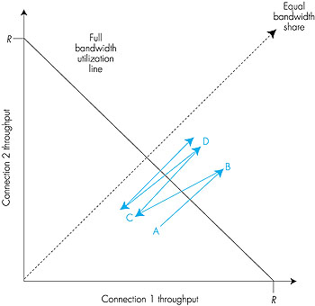
Figure 3.51 plots the throughput realized by the two TCP connections. If TCP is to equally share the link bandwidth between the two connections, then the realized throughput should fall along the 45-degree arrow ("equal bandwidth share") emanating from the origin. Ideally, the sum of the two throughputs should equal R. (Certainly, each connection receiving an equal, but zero, share of the link capacity is not a desirable situation!) So the goal should be to have the achieved throughputs fall somewhere near the intersection of the "equal bandwidth share" line and the "full bandwidth utilization" line in Figure 3.51. 

Suppose that the TCP window sizes are such that at a given point in time, connections 1 and 2 realize throughputs indicated by point A in Figure 3.51. Because the amount of link bandwidth jointly consumed by the two connections is less than R, no loss will occur, and both connections will increase their window by 1 per RTT as a result of TCP's congestion-avoidance algorithm. Thus, the joint throughput of the two connections proceeds along a 45-degree line (equal increase for both connections) starting from point A. Eventually, the link bandwidth jointly consumed by the two connections will be greater than R and eventually packet loss will occur. Suppose that connections 1 and 2 experience packet loss when they realize throughputs indicated by point B. Connections 1 and 2 then decrease their windows by a factor of two. The resulting throughputs realized are thus at point C, halfway along a vector starting at B and ending at the origin. Because the joint bandwidth use is less than R at point C, the two connections again increase their throughputs along a 45-degree line starting from C. Eventually, loss will again occur, for example, at point D, and the two connections again decrease their window sizes by a factor of two, and so on. You should convince yourself that the bandwidth realized by the two connections eventually fluctuates along the equal bandwidth share line. You should also convince yourself that the two connections will converge to this behavior regardless of where they are in the two-dimensional space! Although a number of idealized assumptions lay behind this scenario, it still provides an intuitive feel for why TCP results in an equal sharing of bandwidth among connections. 

In our idealized scenario, we assumed that only TCP connections traverse the bottleneck link, and that only a single TCP connection is associated with a host-destination pair. In practice, these two conditions are typically not met, and client/ server applications can thus obtain very unequal portions of link bandwidth. 

Many network applications run over TCP rather than UDP because they want to make use of TCP's reliable transport service. But an application developer choosing TCP gets not only reliable data transfer but also TCP congestion control. We have just seen how TCP congestion control regulates an application's transmission rate via the congestion-window mechanism. Many multimedia applications do not run over TCP for this very reason--they do not want their transmission rate throttled, even if the network is very congested. In particular, many Internet telephone and Internet video conferencing applications typically run over UDP. These applications prefer to pump their audio and video into the network at a constant rate and occasionally lose packets, rather than reduce their rates to "fair" levels at times of congestion and not lose any packets. From the perspective of TCP, the multimedia applications running over UDP are not being fair--they do not cooperate with the other connections nor adjust their transmission rates appropriately. A major challenge in the upcoming years will be to develop congestion-control mechanisms for the Internet that prevent UDP traffic from bringing the Internet's throughput to a grinding halt, [Floyd 1999]. 

But even if we could force UDP traffic to behave fairly, the fairness problem would still not be completely solved. This is because there is nothing to stop an application running over TCP from using multiple parallel connections. For example, Web browsers often use multiple parallel TCP connections to transfer a Web page. (The exact number of multiple connections is configurable in most browsers.) When an application uses multiple parallel connections, it gets a larger fraction of the bandwidth in a congested link. As an example, consider a link of rate R supporting nine ongoing client/server applications, with each of the applications using one TCP connection. If a new application comes along and also uses one TCP connection, then each application gets approximately the same transmission rate of R/10. But if this new application instead uses 11 parallel TCP connections, then the new application gets an unfair allocation of more than R/2. Because Web traffic is so pervasive in the Internet, multiple parallel connections are not uncommon. 

Macroscopic Description of TCP Dynamics

Consider sending a very large file over a TCP connection. If we take a macroscopic view of the traffic sent by the source, we can ignore the slow-start phase. Indeed, the connection is in the slow-start phase for a relatively short period of time because the connection grows out of the phase exponentially fast. When we ignore the slow-start phase, the congestion window grows linearly, gets chopped in half when loss occurs, grows linearly, gets chopped in half when loss occurs, and so on. This gives rise to the saw-tooth behavior of TCP [Stevens 1994] shown in Figure 3.49. 

Given this saw-tooth behavior, what is the average throughput of a TCP connection? During a particular round-trip interval, the rate at which TCP sends data is a function of the congestion window and the current RTT. When the window size is w • MSS and the current round-trip time is RTT, then TCP's transmission rate is (w • MSS)/RTT. During the congestion-avoidance phase, TCP probes for additional bandwidth by increasing w by one each RTT until loss occurs. (Denote by W the value of w at which loss occurs.) Assuming that RTT and W are approximately constant over the duration of the connection, the TCP transmission rate ranges from 

These assumptions lead to a highly simplified macroscopic model for the steady-state behavior of TCP. The network drops a packet from the connection when the connection's window size increases to W • MSS; the congestion window is then cut in half and then increases by one MSS per round-trip time until it again reaches W. This process repeats itself over and over again. Because the TCP throughput increases linearly between the two extreme values, we have: 

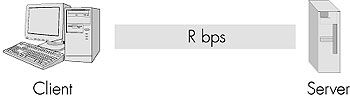
Using this highly idealized model for the steady-state dynamics of TCP, we can also derive an interesting expression that relates a connection's loss rate to its available bandwidth [Mahdavi 1997]. This derivation is outlined in the homework problems. 

3.7.2: Modeling Latency: Static Congestion Window

The analysis presented here assumes that the network is uncongested, that is, that the TCP connection transporting the object does not have to share link bandwidth with other TCP or UDP traffic. (We comment on this assumption below.) Also, in order to not obscure the central issues, we carry out the analysis in the context of the simple one-link network as shown in Figure 3.52. (This link might model a single bottleneck on an end-to-end path. See also the homework problems for an explicit extension to the case of multiple links.) 

We also make the following simplifying assumptions: 

• The amount of data that the sender can transmit is solely limited by the sender's congestion window. (Thus, the TCP receive buffers are large.) 
• Packets are neither lost nor corrupted, so that there are no retransmissions. 
• All protocol header overheads--including TCP, IP, and link-layer headers--are negligible and ignored. 
• The object (that is, file) to be transferred consists of an integer number of segments of size MSS (maximum segment size). 
• The only packets that have non-negligible transmission times are packets that carry maximum-size TCP segments. Request messages, acknowledgments, and TCP connection establishment segments are small and have negligible transmission times. 
• The initial threshold in the TCP congestion-control mechanism is a large value that is never attained by the congestion window.

• The size of the object to be transferred is O bits. 
• The MSS (maximum size segment) is S bits (for example, 536 bytes). 
• The transmission rate of the link from the server to the client is R bps. 
• The round-trip time is denoted by RTT.

Although the analysis presented in this section assumes an uncongested network with a single TCP connection, it nevertheless sheds insight on the more realistic case of multilink congested network. For a congested network, R roughly represents the amount of bandwidth received in steady state in the end-to-end network connection, and RTT represents a round-trip delay that includes queuing delays at the routers preceding the congested links. In the congested network case, we model each TCP connection as a constant-bit-rate connection of rate R bps preceded by a single slow-start phase. (This is roughly how TCP Tahoe behaves when losses are detected with triple duplicate acknowledgments.) In our numerical examples, we use values of R and RTT that reflect typical values for a congested network. 

Before beginning the formal analysis, let us try to gain some intuition. Let us consider what would be the latency if there were no congestion-window constraint; that is, if the server were permitted to send segments back-to-back until the entire object is sent. To answer this question, first note that one RTT is required to initiate the TCP connection. After one RTT, the client sends a request for the object (which is piggybacked onto the third segment in the three-way TCP handshake). After a total of two RTTs, the client begins to receive data from the server. The client receives data from the server for a period of time O/R, the time for the server to transmit the entire object. Thus, in the case of no congestion-window constraint, the total latency is 2 RTT + O/R. This represents a lower bound; the slow-start procedure, with its dynamic congestion window, will of course elongate this latency. 

Static Congestion Window

Although TCP uses a dynamic congestion window, it is instructive to first analyze the case of a static congestion window. Let W, a positive integer, denote a fixed-size static congestion window. For the static congestion window, the server is not permitted to have more than W unacknowledged outstanding segments. When the server receives the request from the client, the server immediately sends W segments back-to-back to the client. The server then sends one segment into the network for each acknowledgment it receives from the client. The server continues to send one segment for each acknowledgment until all of the segments of the object have been sent. There are two cases to consider: 

1. WS/R > RTT + S/R. In this case, the server receives an acknowledgment for the first segment in the first window before the server completes the transmission of the first window. 
2. WS/R < RTT + S/R. In this case, the server transmits the first window's worth of segments before the server receives an acknowledgment for the first segment in the window.

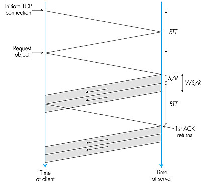
One RTT is required to initiate the TCP connection. After one RTT, the client sends a request for the object (which is piggybacked onto the third segment in the three-way TCP handshake). After a total of two RTTs, the client begins to receive data from the server. Segments arrive periodically from the server every S/R seconds, and the client acknowledges every segment it receives from the server. Because the server receives the first acknowledgment before it completes sending a window's worth of segments, the server continues to transmit segments after having transmitted the first window's worth of segments. And because the acknowledgments arrive periodically at the server every S/R seconds from the time when the first acknowledgment arrives, the server transmits segments continuously until it has transmitted the entire object. Thus, once the server starts to transmit the object at rate R, it continues to transmit the object at rate R until the entire object is transmitted. The latency therefore is 2 RTT + O/R. 

Now let us consider case 2, which is illustrated in Figure 3.54. In this figure, the window size is W = 2 segments. 

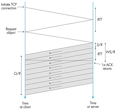
Once again, after a total of two RTTs, the client begins to receive segments from the server. These segments arrive periodically every S/R seconds, and the client acknowledges every segment it receives from the server. But now the server completes the transmission of the first window before the first acknowledgment arrives from the client. Therefore, after sending a window, the server must stall and wait for an acknowledgment before resuming transmission. When an acknowledgment finally arrives, the server sends a new segment to the client. Once the first acknowledgment arrives, a window's worth of acknowledgments arrive, with each successive acknowledgment spaced by S/R seconds. For each of these acknowledgments, the server sends exactly one segment. Thus, the server alternates between two states: a transmitting state, during which it transmits W segments, and a stalled state, during which it transmits nothing and waits for an acknowledgment. The latency is equal to 2 RTT plus the time required for the server to transmit the object, O/R, plus the amount of time that the server is in the stalled state. To determine the amount of time the server is in the stalled state, let K = O/WS; if O/WS is not an integer, then round K up to the nearest integer. Note that K is the number of windows of data there are in the object of size O. The server is in the stalled state between the transmission of each of the windows, that is, for K - 1 periods of time, with each period lasting RTT - (W - 1)S/R (see Figure 3.54). Thus, for case 2, 

Combining the two cases, we obtain 

where [x]⁺ = max(x,0). 

This completes our analysis of static windows. The following analysis for dynamic windows is more complicated, but parallels that for static windows. 

3.7.3: Modeling Latency: Dynamic Congestion Window

Note that O/S is the number of segments in the object; in the above diagram, O/S = 15. Consider the number of segments that are in each of the windows. The first window contains one segment, the second window contains two segments, and the third window contains four segments. More generally, the kth window contains 2^k-1 segments. Let K be the number of windows that cover the object; in the preceding diagram, K = 4. In general, we can express K in terms of O/S as follows: 

After transmitting a window's worth of data, the server may stall (that is, stop transmitting) while it waits for an acknowledgment. In Figure 3.55, the server stalls after transmitting the first and second windows, but not after transmitting the third. Let us now calculate the amount of stall time after transmitting the kth window. The time the server begins to transmit the kth window until the time when the server receives an acknowledgment for the first segment in the window is S/R + RTT. The transmission time of the kth window is (S/R) 2^k-1. The stall time is the difference of these two quantities, that is, 

The server can potentially stall after the transmission of each of the first k - 1 windows. (The server is done after the transmission of the kth window.) We can now calculate the latency for transferring the file. The latency has three components: 2 RTT for setting up the TCP connection and requesting the file, O/R, the transmission time of the object, and the sum of all the stalled times. Thus, 

The reader should compare the above equation for the latency equation for static congestion windows; all the terms are exactly the same except that the term WS/R for static windows has been replaced by 2^k-1(S/R) for dynamic windows. To obtain a more compact expression for the latency, let Q be the number of times the server would stall if the object contained an infinite number of segments: 

The actual number of times the server stalls is P = min{Q,K-1}. In Figure 3.55, P = Q = 2. Combining the above two equations gives 

We can further simplify the above formula for latency by noting 

Combining the above two equations gives the following closed-form expression for the latency: 

Thus to calculate the latency, we simply must calculate K and Q, set P = min {Q,K-1}, and plug P into the above formula. 

It is interesting to compare the TCP latency to the latency that would occur if there were no congestion control (that is, no congestion window constraint). Without congestion control, the latency is 2 RTT + O/R, which we define to be the minimum latency. It is a simple exercise to show that 

We see from the above formula that TCP slow start will not significantly increase latency if RTT << O/R, that is, if the round-trip time is much less than the transmission time of the object. Thus, if we are sending a relatively large object over an uncongested high-speed link, then slow start has an insignificant effect on latency. However, with the Web, we are often transmitting many small objects over congested links, in which case slow start can significantly increase latency (as we'll see in the following subsection). 

Let us now take a look at some example scenarios. In all the scenarios we set S = 536 bytes, a common default value for TCP. We'll use an RTT of 100 msec, which is not an atypical value for a continental or intercontinental delay over moderately congested links. First consider sending a rather large object of size O = 100 Kbytes. The number of windows that cover this object is K = 8. For a number of transmission rates, the following table examines the effect of the slow-start mechanism on the latency. 

R	O/R	P	Minimum Latency: O/R + 2 RTT	Latency with slow start
28 Kbps	28.6 sec	1	28.8 sec	28.9 sec
100 Kbps	8 sec	2	8.2 sec	8.4 sec
1 Mbps	800 msec	5	1 sec	1.5 sec
10 Mbps	80 msec	7	0.28 sec	0.98 sec

We see from the above chart that for a large object, slow-start adds appreciable delay only when the transmission rate is high. If the transmission rate is low, then acknowledgments come back relatively quickly, and TCP quickly ramps up to its maximum rate. For example, when R = 100 Kbps, the number of stall periods is P = 2 whereas the number of windows to transmit is K = 8; thus the server stalls only after the first two of eight windows. On the other hand, when R = 10 Mbps, the server stalls between each window, which causes a significant increase in the delay. 

Now consider sending a small object of size O = 5 Kbytes. The number of windows that cover this object is K = 4. For a number of transmission rates, the following table examines the effect of the slow-start mechanism. 

R	O/R	P	Minimum latency: O/R + 2 RTT	Latency with slow start
28 Kbps	1.43 sec	1	1.63 sec	1.73 sec
100 Kbps	0.4 sec	2	0.6 sec	0.757 sec
1 Mbps	40 msec	3	0.24 sec	0.52 sec
10 Mbps	4 msec	3	0.20 sec	0.50 sec

Once again, slow start adds an appreciable delay when the transmission rate is high. For example, when R = 1 Mbps, the server stalls between each window, which causes the latency to be more than twice that of the minimum latency. 

For a larger RTT, the effect of slow start becomes significant for small objects for smaller transmission rates. The following table examines the effect of slow start for RTT = 1 second and O = 5 Kbytes (K = 4). 

R	O/R	P	Minimum latency: O/R + 2 RTT	Latency with slow start
28 Kbps	1.43 sec	3	3.4 sec	5.8 sec
100 Kbps	0.4 sec	3	2.4 sec	5.2 sec
1 Mbps	40 msec	3	2.0 sec	5.0 sec
10 Mbps	4 msec	3	2.0 sec	5.0 sec

In summary, slow start can significantly increase latency when the object size is relatively small and the RTT is relatively large. Unfortunately, this is often the scenario when sending objects over the World Wide Web. 

An Example: HTTP

As an application of the latency analysis, let's now calculate the response time for a Web page sent over nonpersistent HTTP. Suppose that the page consists of one base HTML page and M referenced images. To keep things simple, let us assume that each of the M + 1 objects contains exactly O bits. 

With nonpersistent HTTP, each object is transferred independently, one after the other. The response time of the Web page is therefore the sum of the latencies for the individual objects. Thus 

Note that the response time for nonpersistent HTTP takes the form: 

Clearly, if there are many objects in the Web page and if RTT is large, then non-persistent HTTP will have poor response-time performance. In the homework problems, we will investigate the response time for other HTTP transport schemes, including persistent connections and nonpersistent connections with parallel connections. The reader is also encouraged to see [Heidemann 1997] for a related analysis.