Real-time interactive multimedia applications, such as Internet phone and real-time video conferencing, are acutely sensitive to packet delay, jitter, and loss. Fortunately, designers of these applications can introduce several useful mechanisms that can preserve good audio and video quality as long as delay, jitter, and loss are not excessive. In this section, we examine some of these mechanisms. To keep the discussion concrete, we discuss these mechanisms in the context of an Internet phone application, described below. The situation is similar for real-time video conferencing applications [Bolot 1994]. 

The speaker in our Internet phone application generates an audio signal consisting of alternating talk spurts and silent periods. In order to conserve bandwidth, our Internet phone application only generates packets during talk spurts. During a talk spurt the sender generates bytes at a rate of 8 Kbytes per second, and every 20 milliseconds the sender gathers bytes into chunks. Thus, the number of bytes in a chunk is (20 msecs) · (8 Kbytes/sec) = 160 bytes. A special header is attached to each chunk, the contents of which is discussed below. The chunk and its header are encapsulated in a UDP segment, and then the UDP datagram is sent into the socket interface. Thus, during a talk spurt, a UDP segment is sent every 20 msec. 

If each packet makes it to the receiver and has a small constant end-to-end delay, then packets arrive at the receiver periodically every 20 msec during a talk spurt. In these ideal conditions, the receiver can simply play back each chunk as soon as it arrives. But, unfortunately, some packets can be lost and most packets will not have the same end-to-end delay, even in a lightly congested Internet. For this reason, the receiver must take more care in (1) determining when to play back a chunk, and (2) determining what to do with a missing chunk. 

6.3.1: The Limitations of a Best-Effort Service

Packet Loss

Consider one of the UDP segments generated by our Internet phone application. The UDP segment is encapsulated in an IP datagram. As the datagram wanders through the network, it passes through buffers (that is, queues) in the routers in order to access outbound links. It is possible that one or more of the buffers in the route from sender to receiver is full and cannot admit the IP datagram. In this case, the IP datagram is discarded, never to arrive at the receiving application. 

Loss could be eliminated by sending the packets over TCP rather than over UDP. Recall that TCP retransmits packets that do not arrive at the destination. However, retransmission mechanisms are often considered unacceptable for interactive real-time audio applications such as Internet phone, because they increase end-to-end delay [Bolot 1996]. Furthermore, due to TCP congestion control, after packet loss the transmission rate at the sender can be reduced to a rate that is lower than the drain rate at the receiver. This can have a severe impact on voice intelligibility at the receiver. For these reasons, almost all existing Internet phone applications run over UDP and do not bother to retransmit lost packets. 

But losing packets is not necessarily as grave as one might think. Indeed, packet loss rates between 1% and 20% can be tolerated, depending on how the voice is encoded and transmitted, and on how the loss is concealed at the receiver. For example, forward error correction (FEC) can help conceal packet loss. We'll see below that with FEC, redundant information is transmitted along with the original information so that some of the lost original data can be recovered from the redundant information. Nevertheless, if one or more of the links between sender and receiver is severely congested, and packet loss exceeds 10-20%, then there is really nothing that can be done to achieve acceptable sound quality. Clearly, best-effort service has its limitations. 

End-to-End Delay

End-to-end delay is the accumulation of transmission processing and queuing delays in routers, propagation delays, and end-system processing delays along a path from source to destination. For highly interactive audio applications, such as Internet phone, end-to-end delays smaller than 150 milliseconds are not perceived by a human listener; delays between 150 and 400 milliseconds can be acceptable but not ideal; and delays exceeding 400 milliseconds can seriously hinder the interactivity in voice conversations. The receiver in an Internet phone application will typically disregard any packets that are delayed more than a certain threshold, for example, more than 400 milliseconds. Thus, packets that are delayed by more than the threshold are effectively lost. 

Delay Jitter

A crucial component of end-to-end delay is the random queuing delays in the routers. Because of these varying delays within the network, the time from when a packet is generated at the source until it is received at the receiver can fluctuate from packet to packet. This phenomenon is called jitter.

As an example, consider two consecutive packets within a talk spurt in our Internet phone application. The sender sends the second packet 20 msec after sending the first packet. But at the receiver, the spacing between these packets can become greater than 20 msec. To see this, suppose the first packet arrives at a nearly empty queue at a router, but just before the second packet arrives at the queue a large number of packets from other sources arrive to the same queue. Because the second packet suffers a large queuing delay, the first and second packets become spaced apart by more than 20 msecs. The spacing between consecutive packets can also become less than 20 msecs. To see this, again consider two consecutive packets within a talk spurt. Suppose the first packet joins the end of a queue with a large number of packets, and the second packet arrives at the queue before packets from other sources arrive at the queue. In this case, our two packets find themselves right behind each other in the queue. If the time it takes to transmit a packet on the router's inbound link is less than 20 msecs, then the first and second packets become spaced apart by less than 20 msecs. 

The situation is analogous to driving cars on roads. Suppose you and your friend are each driving in your own cars from San Diego to Phoenix. Suppose you and your friend have similar driving styles, and that you both drive at 100 km/ hour, traffic permitting. Finally, suppose your friend starts out one hour before you. Then, depending on intervening traffic, you may arrive at Phoenix more or less than one hour after your friend. 

If the receiver ignores the presence of jitter, and plays out chunks as soon as they arrive, then the resulting audio quality can easily become unintelligible at the receiver. Fortunately, jitter can often be removed by using sequence numbers, timestamps, and a playout delay, as discussed below. 

6.3.2: Removing Jitter at the Receiver for Audio

• Prefacing each chunk with a sequence number. The sender increments the sequence number by one for each of the packet it generates. 
• Prefacing each chunk with a timestamp. The sender stamps each chunk with the time at which the chunk was generated. 
• Delaying playout of chunks at the receiver. The playout delay of the received audio chunks must be long enough so that most of the packets are received before their scheduled playout times. This playout delay can either be fixed throughout the duration of the conference, or it may vary adaptively during the conference's lifetime. Packets that do not arrive before their scheduled playout times are considered lost and forgotten; as noted above, the receiver may use some form of speech interpolation to attempt to conceal the loss.

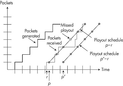
Fixed Playout Delay

With the fixed delay strategy, the receiver attempts to playout each chunk exactly q msecs after the chunk is generated. So if a chunk is timestamped at time t, the receiver plays out the chunk at time t + q, assuming the chunk has arrived by that time. Packets that arrive after their scheduled playout times are discarded and considered lost. 

What is a good choice for q? Internet telephone can support delays up to about 400 msecs, although a more satisfying interactive experience is achieved with smaller values of q. On the other hand, if q is made much smaller than 400 msecs, then many packets may miss their scheduled playback times due to the network-induced delay jitter. Roughly speaking, if large variations in end-to-end delay are typical, it is preferable to use a large q; on the other hand, if delay is small and variations in delay are also small, it is preferable to use a small q, perhaps less than 150 msecs. 

The tradeoff between the playback delay and packet loss is illustrated in Figure 6.6. The figure shows the times at which packets are generated and played out for a single talkspurt. Two distinct initial playout delays are considered. As shown by the leftmost staircase, the sender generates packets at regular intervals--say, every 20 msec. The first packet in this talkspurt is received at time r. As shown in the figure, the arrivals of subsequent packets are not evenly spaced due to the network jitter. 

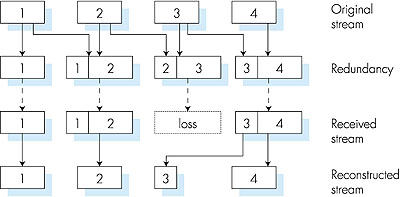
For the first playout schedule, the fixed initial playout delay is set to p - r. With this schedule, the fourth packet does not arrive by its scheduled playout time, and the receiver considers it lost. For the second playout schedule, the fixed initial playout delay is set to p' - r. For this schedule, all packets arrive before their scheduled playout times, and there is therefore no loss. 

Adaptive Playout Delay

The above example demonstrates an important delay-loss tradeoff that arises when designing a playout strategy with fixed playout delays. By making the initial playout delay large, most packets will make their deadlines and there will therefore be negligible loss; however, for interactive services such as Internet phone, long delays can become bothersome if not intolerable. Ideally, we would like the play-out delay to be minimized subject to the constraint that the loss be below a few percent. 

The natural way to deal with this tradeoff is to estimate the network delay and the variance of the network delay, and to adjust the playout delay accordingly at the beginning of each talkspurt. This adaptive adjustment of playout delays at the beginning of the talkspurts will cause the sender's silent periods to be compressed and elongated; however, compression and elongation of silence by a small amount is not noticeable in speech. 

Following [Ramjee 1994], we now describe a generic algorithm that the receiver can use to adaptively adjust its playout delays. To this end, let 

t_i = timestamp of the ith packet = the time packet was generated by sender 

r_i = the time packet i is received by receiver 

p_i = the time packet i is played at receiver 

The end-to-end network delay of the ith packet is r_i - t_i. Due to network jitter, this delay will vary from packet to packet. Let d_i denote an estimate of the average network delay upon reception of the ith packet. This estimate is constructed from the timestamps as follows: 

where u is a fixed constant (for example, u = 0.01). Thus d_i is a smoothed average of the observed network delays r₁ - t₁, . . . , r_i - t_i. The estimate places more weight on the recently observed network delays than on the observed network delays of the distant past. This form of estimate should not be completely unfamiliar; a similar idea is used to estimate round-trip times in TCP, as discussed in Chapter 3. Let v_i denote an estimate of the average deviation of the delay from the estimated average delay. This estimate is also constructed from the timestamps: 

The estimates d_i and v_i are calculated for every packet received, although they are only used to determine the playout point for the first packet in any talkspurt. 

Once having calculated these estimates, the receiver employs the following algorithm for the playout of packets. If packet i is the first packet of a talkspurt, its playout time, p_i, is computed as: 

where K is a positive constant (for example, K = 4). The purpose of the Kv_i term is to set the playout time far enough into the future so that only a small fraction of the arriving packets in the talkspurt will be lost due to late arrivals. The playout point for any subsequent packet in a talkspurt is computed as an offset from the point in time when the first packet in the talkspurt was played out. In particular, let 

be the length of time from when the first packet in the talkspurt is generated until it is played out. If packet j also belongs to this talkspurt, it is played out at time 

The algorithm just described makes perfect sense assuming that the receiver can tell whether a packet is the first packet in the talkspurt. If there is no packet loss, then the receiver can determine whether packet i is the first packet of the talkspurt by comparing the timestamp of the ith packet with the timestamp of the (i - 1)st packet. Indeed, if t_i - t_i-1 > 20 msec, then the receiver knows that ith packet starts a new talkspurt. But now suppose there is occasional packet loss. In this case, two successive packets received at the destination may have timestamps that differ by more than 20 msec when the two packets belong to the same talkspurt. So here is where the sequence numbers are particularly useful. The receiver can use the sequence numbers to determine whether a difference of more than 20 msec in timestamps is due to a new talkspurt or to lost packets. 

6.3.3: Recovering from Packet Loss

As mentioned at the beginning of this section, retransmitting lost packets is not appropriate in an interactive real-time application such as Internet phone. Indeed, retransmitting a packet that has missed its playout deadline serves absolutely no purpose. And retransmitting a packet that overflowed a router queue cannot normally be accomplished quickly enough. Because of these considerations, Internet phone applications often use some type of loss anticipation scheme. Two types of loss-anticipation schemes are forward error correction (FEC) and interleaving.

Forward Error Correction (FEC) 

The basic idea of FEC is to add redundant information to the original packet stream. For the cost of marginally increasing the transmission rate of the audio of the stream, the redundant information can be used to reconstruct "approximations" or exact versions of some of the lost packets. Following [Bolot 1996] and [Perkins 1998], we now outline two FEC mechanisms. The first mechanism sends a redundant encoded chunk after every n chunks. The redundant chunk is obtained by exclusive OR-ing the n original chunks [Shacham 1990]. In this manner if any one packet of the group of n + 1 packets is lost, the receiver can fully reconstruct the lost packet. But if two or more packets in a group are lost, the receiver cannot reconstruct the lost packets. By keeping n + 1, the group size, small, a large fraction of the lost packets can be recovered when loss is not excessive. However, the smaller the group size, the greater the relative increase of the transmission rate of the audio stream. In particular, the transmission rate increases by a factor of 1/n; for example, if n = 3, then the transmission rate increases by 33%. Furthermore, this simple scheme increases the playout delay, as the receiver must wait to receive the entire group of packets before it can begin playout. 

The second FEC mechanism is to send a lower-resolution audio stream as the redundant information. For example, the sender might create a nominal audio stream and a corresponding low-resolution low-bit rate audio stream. (The nominal stream could be a PCM encoding at 64 Kbps and the lower-quality stream could be a GSM encoding at 13 Kbps.) The low-bit-rate stream is referred to as the redundant stream. As shown in Figure 6.7, the sender constructs the nth packet by taking the nth chunk from the nominal stream and appending to it the (n - 1)st chunk from the redundant stream. In this manner, whenever there is nonconsecutive packet loss, the receiver can conceal the loss by playing out the low-bit-rate encoded chunk that arrives with the subsequent packet. Of course, low-bit-rate chunks give lower quality than the nominal chunks. However, a stream of mostly high-quality chunks, occasional low-quality chunks, and no missing chunks gives good overall audio quality. Note that in this scheme, the receiver only has to receive two packets before playback, so that the increased playout delay is small. Furthermore, if the low-bit-rate encoding is much less than the nominal encoding, then the marginal increase in the transmission rate will be small. 

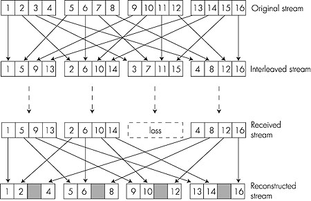
In order to cope with consecutive loss, a simple variation can be employed. Instead of appending just the (n - 1)st low-bit-rate chunk to the nth nominal chunk, the sender can append the (n - 1)st and (n - 2)nd low-bit-rate chunk, or append the (n - 1)st and (n - 3)rd low-bit-rate chunk, etc. By appending more low-bit-rate chunks to each nominal chunk, the audio quality at the receiver becomes acceptable for a wider variety of harsh best-effort environments. On the other hand, the additional chunks increase the transmission bandwidth and the playout delay. 

Free Phone [Freephone 1999] and RAT [RAT 1999] are well-documented Internet phone applications that use FEC. They can transmit lower-quality audio streams along with the nominal audio stream, as described above. 

Interleaving

As an alternative to redundant transmission, an Internet phone application can send interleaved audio. As shown in Figure 6.8, the sender resequences units of audio data before transmission, so that originally adjacent units are separated by a certain distance in the transmitted stream. Interleaving can mitigate the effect of packet losses. If, for example, units are 5 msec in length and chunks are 20 msec (that is, 4 units per chunk), then the first chunk could contain units 1, 5, 9, 13; the second chunk could contain units 2, 6, 10, 14; and so on. Figure 6.8 shows that the loss of a single packet from an interleaved stream results in multiple small gaps in the reconstructed stream, as opposed to the single large gap that would occur in a noninterleaved stream. 

Interleaving can significantly improve the perceived quality of an audio stream [Perkins 1998]. It also has low overhead. The obvious disadvantage of interleaving is that it increases latency. This limits its use for interactive applications such as Internet phone, although it can perform well for streaming stored audio. A major advantage of interleaving is that it does not increase the bandwidth requirements of a stream. 

Receiver-Based Repair of Damaged Audio Streams

Receiver-based recovery schemes attempt to produce a replacement for a lost packet that is similar to the original. As discussed in [Perkins 1998], this is possible since audio signals, and in particular speech, exhibit large amounts of short-term self similarity. As such, these techniques work for relatively small loss rates (less than 15%), and for small packets (4-40 msec). When the loss length approaches the length of a phoneme (5-100 msec) these techniques breakdown, since whole phonemes may be missed by the listener. 

Perhaps the simplest form of receiver-based recovery is packet repetition. Packet repetition replaces lost packets with copies of the packets that arrived immediately before the loss. It has low computational complexity and performs reasonably well. Another form of receiver-based recovery is interpolation, which uses audio before and after the loss to interpolate a suitable packet to cover the loss. It performs somewhat better than packet repetition, but is significantly more computationally intensive [Perkins 1998]. 

6.3.4: Streaming Stored Audio and Video