6.6.1: Scheduling Mechanisms

First-In-First-Out (FIFO) 

Figure 6.23 shows the queuing model abstractions for the First-in-First-Out (FIFO) link scheduling discipline. Packets arriving at the link output queue are queued for transmission if the link is currently busy transmitting another packet. If there is not sufficient buffering space to hold the arriving packet, the queue's packet discarding policy then determines whether the packet will be dropped ("lost") or whether other packets will be removed from the queue to make space for the arriving packet. In our discussion below we will ignore packet discard. When a packet is completely transmitted over the outgoing link (that is, receives service) it is removed from the queue. 

The FIFO scheduling discipline (also known as First-Come-First-Served--FCFS) selects packets for link transmission in the same order in which they arrived at the output link queue. We're all familiar with FIFO queuing from bus stops (particularly in England, where queuing seems to have been perfected) or other service centers, where arriving customers join the back of the single waiting line, remain in order, and are then served when they reach the front of the line. 

Figure 6.24 shows an example of the FIFO queue in operation. Packet arrivals are indicated by numbered arrows above the upper timeline, with the number indicating the order in which the packet arrived. Individual packet departures are shown below the lower timeline. The time that a packet spends in service (being transmitted) is indicated by the shaded rectangle between the two timelines. Because of the FIFO discipline, packets leave in the same order in which they arrived. Note that after the departure of packet 4, the link remains idle (since packets 1 through 4 have been transmitted and removed from the queue) until the arrival of packet 5. 

Priority Queuing

Under priority queuing, packets arriving at the output link are classified into one of two or more priority classes at the output queue, as shown in Figure 6.25. As discussed in the previous section, a packet's priority class may depend on an explicit marking that it carries in its packet header (for example, the value of the Type of Service (ToS) bits in an IPv4 packet), its source or destination IP address, its destination port number, or other criteria. Each priority class typically has its own queue. When choosing a packet to transmit, the priority queuing discipline will transmit a packet from the highest priority class that has a nonempty queue (that is, has packets waiting for transmission). The choice among packets in the same priority class is typically done in a FIFO manner. 

Figure 6.26 illustrates the operation of a priority queue with two priority classes. Packets 1, 3, and 4 belong to the high-priority class and packets 2 and 5 belong to the low-priority class. Packet 1 arrives and, finding the link idle, begins transmission. During the transmission of packet 1, packets 2 and 3 arrive and are queued in the low- and high-priority queues, respectively. After the transmission of packet 1, packet 3 (a high-priority packet) is selected for transmission over packet 2 (which, even though it arrived earlier, is a low-priority packet). At the end of the transmission of packet 3, packet 2 then begins transmission. Packet 4 (a high-priority packet) arrives during the transmission of packet 3 (a low-priority packet). Under a so-called non-preemptive priority queuing discipline, the transmission of a packet is not interrupted once it has begun. In this case, packet 4 queues for transmission and begins being transmitted after the transmission of packet 2 is completed. 

Round Robin and Weighted Fair Queuing (WFQ) 

Under the round robin queuing discipline, packets are again sorted into classes, as with priority queuing. However, rather than there being a strict priority of service among classes, a round robin scheduler alternates service among the classes. In the simplest form of round robin scheduling, a class 1 packet is transmitted, followed by a class 2 packet, followed by a class 1 packet, followed by a class 2 packet, and so on. A so-called work-conserving queuing discipline will never allow the link to remain idle whenever there are packets (of any class) queued for transmission. A work-conserving round robin discipline that looks for a packet of a given class but finds none will immediately check the next class in the round robin sequence. 

Figure 6.27 illustrates the operation of a two-class round robin queue. In this example, packets 1, 2, and 4 belong to class 1, and packets 3 and 5 belong to the second class. Packet 1 begins transmission immediately upon arrival at the output queue. Packets 2 and 3 arrive during the transmission of packet 1 and thus queue for transmission. After the transmission of packet 1, the link scheduler looks for a class-2 packet and thus transmits packet 3. After the transmission of packet 3, the scheduler looks for a class-1 packet and thus transmits packet 2. After the transmission of packet 2, packet 4 is the only queued packet; it is thus transmitted immediately after packet 2. 

A generalized abstraction of round robin queuing that has found considerable use in QoS architectures is the so-called weighted fair queuing (WFQ) discipline [Demers 1990; Parekh 1993]. WFQ is illustrated in Figure 6.28. Arriving packets are again classified and queued in the appropriate per-class waiting area. As in round robin scheduling, a WFQ scheduler will again serve classes in a circular manner--first serving class 1, then serving class 2, then serving class 3, and then (assuming there are three classes) repeating the service pattern. WFQ is also a work-conserving queuing discipline and thus will immediately move on to the next class in the service sequence upon finding an empty class queue. 

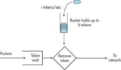
WFQ differs from round robin in that each class may receive a differential amount of service in any interval of time. Specifically, each class, i, is assigned a weight, w_i. Under WFQ, during any interval of time during which there are class i packets to send, class i will then be guaranteed to receive a fraction of service equal to w_i/(w_j), where the sum in the denominator is taken over all classes that also have packets queued for transmission. In the worst case, even if all classes have queued packets, class i will still be guaranteed to receive a fraction w_i/(w_j) of the bandwidth. Thus, for a link with transmission rate R, class i will always achieve a throughput of at least R · w_i/(w_j). Our description of WFQ has been an idealized one, as we have not considered the fact that packets are discrete units of data and a packet's transmission will not be interrupted to begin transmission of another packet; [Demers 1990] and [Parekh 1993] discuss this packetization issue. As we will see in the following sections, WFQ plays a central role in QoS architectures. It is also available in today's router products [Cisco QoS 1997]. (Intranets that use WFQ-capable routers can therefore provide QoS to their internal flows.) 

6.6.2: Policing: The Leaky Bucket

• Average rate. The network may wish to limit the long-term average rate (packets per time interval) at which a flow's packets can be sent into the network. A crucial issue here is the interval of time over which the average rate will be policed. A flow whose average rate is limited to 100 packets per second is more constrained than a source that is limited to 6,000 packets per minute, even though both have the same average rate over a long enough interval of time. For example, the latter constraint would allow a flow to send 1,000 packets in a given second-long interval of time (subject to the constraint that the rate be less than 6,000 packets over a minute-long interval containing these 1,000 packets), while the former constraint would disallow this sending behavior. 
• Peak rate. While the average rate-constraint limits the amount of traffic that can be sent into the network over a relatively long period of time, a peak-rate constraint limits the maximum number of packets that can be sent over a shorter period of time. Using our example above, the network may police a flow at an average rate of 6,000 packets per minute, while limiting the flow's peak rate to 1,500 packets per second. 
• Burst size. The network may also wish to limit the maximum number of packets (the "burst" of packets) that can be sent into the network over an extremely short interval of time. In the limit, as the interval length approaches zero, the burst size limits the number of packets that can be instantaneously sent into the network. Even though it is physically impossible to instantaneously send multiple packets into the network (after all, every link has a physical transmission rate that cannot be exceeded!), the abstraction of a maximum burst size is a useful one.

Let us now consider how the leaky bucket can be used to police a packet flow. Suppose that before a packet is transmitted into the network, it must first remove a token from the token bucket. If the token bucket is empty, the packet must wait for a token. (An alternative is for the packet to be dropped, although we will not consider that option here.) Let us now consider how this behavior polices a traffic flow. Because there can be at most b tokens in the bucket, the maximum burst size for a leaky-bucket-policed flow is b packets. Furthermore, because the token generation rate is r, the maximum number of packets that can enter the network of any interval of time of length t is rt + b. Thus, the token generation rate, r, serves to limit the long-term average rate at which the packet can enter the network. It is also possible to use leaky buckets (specifically, two leaky buckets in series) to police a flow's peak rate in addition to the long-term average rate; see the homework problems at the end of this chapter. 

Leaky Bucket + Weighted Fair Queuing Provides Provable Maximum Delay in a Queue

In Sections 6.7 and 6.9 we will examine the so-called Intserv and Diffserv approaches for providing quality of service in the Internet. We will see that both leaky bucket policing and WFQ scheduling can play an important role. Let us thus close this section by considering a router's output that multiplexes n flows, each policed by a leaky bucket with parameters b_i and r_i, i = 1, . . . , n, using WFQ scheduling. We use the term "flow" here loosely to refer to the set of packets that are not distinguished from each other by the scheduler. In practice, a flow might be comprised of traffic from a single end-to-end connection (as in Intserv) or a collection of many such connections (as in Diffserv), see Figure 6.30. 

Recall from our discussion of WFQ that each flow, i, is guaranteed to receive a share of the link bandwidth equal to at least R · w_i/(w_j), where R is the transmission rate of the link in packets/sec. What then is the maximum delay that a packet will experience while waiting for service in the WFQ (that is, after passing through the leaky bucket)? Let us focus on flow 1. Suppose that flow 1's token bucket is initially full. A burst of b₁ packets then arrives to the leaky bucket policer for flow 1. These packets remove all of the tokens (without wait) from the leaky bucket and then join the WFQ waiting area for flow 1. Since these b₁ packets are served at a rate of at least R · w₁/(w_j) packet/sec., the last of these packets will then have a maximum delay, d_max, until its transmission is completed, where 

The justification of this formula is that if there are b₁ packets in the queue and packets are being serviced (removed) from the queue at a rate of at least R · w₁/ (w_j) packets per second, then the amount of time until the last bit of the last packet is transmitted cannot be more than b₁/(R · w₁/(w_j)). A homework problem asks you to prove that as long as r₁ < R · w₁/(w_j), then d_max is indeed the maximum delay that any packet in flow 1 will ever experience in the WFQ queue.